Gistemp rose from 0.79°C in December to 0.92°C in January. That is quite similar to TempLS mesh, where the rise has come back to 0.094°C. There were also similar rises in NCEP/NCAR and the satellite indices.
As with the other indices, this is very warm. It is almost the highest anomaly for any month before Oct 2015 (Jan 07 at 0.96°C was higher). And according to NCEP/NCAR, February so far is even warmer.
I'll show the regular GISS plot and TempLS comparison below the fold
Thursday, February 16, 2017
Wednesday, February 15, 2017
Changes to Moyhu latest monthly temperature table.
A brief note - I have changed the format of the latest monthly data table. The immediate thing to notice is that it starts with latest month at the top.
Before there were two tables - last six months of some commonly quoted datasets, and below a larger table of data back to start 2013, with more datasets included. This was becoming unwieldy.
Now there is just one table going back to 2013, but starting at the latest month, so you have to scroll down for earlier times. It has those most commonly quoted sets, but there are buttons at the top that you can click to get a similar table of other subsets. "Main" is the start table; "TempLS" has a collection (coming) of other styles of integration, and also results with adjusted GHCN.
I'm gradually moving RSS V4 TTT to replace the deprecated V3 TLT. I'm still rearranging the order of columns somewhat. There is reorganisation happening behind the scenes.
Monday, February 13, 2017
Spatial distribution of flutter in GHCN adjustment.
I posted recently on flutter in GHCN adjustment. This is the tendency of the Pairwise Homogenisation Algorithm (PHA) to produce short-term fluctuations in monthly adjustments. It arose on a recent discussion of the kerfuffle of John Bates and the Karl 2015 paper, and has been investigated by Peter O'Neill, who is currently posting on the topic. In my earlier post, I looked at the distribution of individual month adjustments, and noted that with generally zero mean, they would be heavily damped on averaging.
But I was curious about the mechanics, so here I compare the same two adjusted files (June 2015 and Feb 9 2017) collected by station. I'll show a histogram, but more interesting is the spatial distribution shown on a trackball sphere map. The histogram shows a distribution of station RMS values tapering rather rapidly toward 1°C. The map shows the flutter is strongly associated with remoteness, especially islands.
Update: I have now enabled clicking to show not only the name of the nearest station, but the RMS adjustment change there in °C. I have also adopted William's suggestion about the color scheme (white for zero, red for large).
Friday, February 10, 2017
January global surface temperature up 0.155°C.
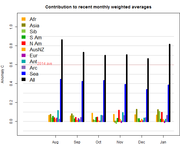
TempLS mesh rose significantly in January, from 0.66°C to 0.815°C. This follows the earlier very similar rise of 0.13°C in the NCEP/NCAR index, and rises in the satellite indices, including a 0.18°C rise in the RSS index. January was the warmest month since April, and as with NCEP/NCAR, it was warmer (in anomaly) than any month before October 2015.
TempLS grid also rose by 0.12°C. I think this month temperatures were not greatly affected by the poles. The breakdown plot was interesting, with contributions to warmth from N America, Asia, Siberia and Africa, with Arctic also warm as usual lately.
TempLS grid also rose by 0.12°C. I think this month temperatures were not greatly affected by the poles. The breakdown plot was interesting, with contributions to warmth from N America, Asia, Siberia and Africa, with Arctic also warm as usual lately.
Thursday, February 9, 2017
Flutter in GHCN V3 adjusted temperatures.
In the recent discussion of the kerfuffle of John Bates and the Karl 2015 paper, the claim of Bates that the GHCN adjustment algorithm was subject to instability arose. Bates claim seemed to be of an actual fault in the code. I explained why I think that is unlikely, but rather it is a feature of the Pairwise Homogenisation Algorithm (PHA).
GHCN V3 adjusted is issued approximately daily, although it is not clear how often the underlying algorithm is run. It is posted here - see the readme file and look for the qca label.
Paul Matthews linked to his analysis of variations in Alice Springs adjusted over time. It did look remarkable; fluctuations of a degree or more over quite short intervals, with maximum excursions of about 3°C. This was in about 2012. However Peter O'Neill had done a much more extensive study with many stations and more recent years (and using many more adjustment files). He found somewhat smaller variations, and of frequent but variable occurrence.
I don't have a succession of GHCN adjusted files available, but I do have the latest (downloaded 9 Feb) and I have one with a file date here of 21 June 2015. So I thought I would look at differences between these to try to get an overall picture of what is going on.
Friday, February 3, 2017
NCEP/NCAR January warmest month since April 2016.
The Moyhu NCEP/NCAR index at 0.486°C was warmer than any month since April 2016. But it was a wild ride. It started very warm, dropped to temperatures lower than seen for over a year, rose again, and the last two weeks were very warm, and it still is. The big dip coincided with the cold snap in E North America, and in Central and East Europe, extending through Russia. Then N America warmed a little, although some of Europe stayed cold, and there was the famous snow in the Sahara. Overall, Arctic and Canada (despite cold snaps) were warm, as was most of Asia. Europe and the Sahara were indeed cold.
I'll note just how warm it still is, historically. I don't make too much of long term records in the reanalysis data, since it can't really be made homogeneous. But January was not only warmest since April, but warmer (by a lot) than any month prior to October 2015.
UAH satellite, which dropped severely in December, rose a little, from 0.24°C to 0.30°C. Arctic sea ice, which had been very low, recovered a bit to be occasionally not the lowest recorded for the time of year. Antarctic ice is still very low, and may well reach a notable minimum.
With the Arctic still warm, I would expect a substantial rise for GISS and TempLS mesh, with maybe less for HADCRUT and NOAA.
Wednesday, February 1, 2017
Homogenisation and Cape Town.
An old perennial in climate wars is the adjustment of land temperature data. Stations are subject to various changes, like moving, which leads to sustained jumps that are not due to climate. For almost any climate analysis that matters, these station records are taken to be representative of some region, so it is important to adjust for the effect of these events. So GHCN publishes an additional list of adjusted temperatures. They are called homogenised with the idea that as far as can be achieved, temperatures from different times are as if measured under like conditions. I have written about this frequently, eg here, here and here.
The contrarian tactic is to find some station that has been changed and beat the drum about rewriting history, or some such. It is usually one where the trend has changed from negative to positive. Since adjustment does change values, this can easily happen. I made a Google Maps gadget here which lets you see how the various GHCN gadgets are affected, and posted histograms here. This blog started its life following a classic 2009 WUWT sally here, based on Darwin. That was probably the most publicised case.
There have been others, and their names are bandied around in skeptic circles as if they were Agincourt and Bannockburn. Jennifer Marohasy has for some reason an irrepressible bee in her bonnet about Rutherglen, and I think we'll be hearing more of it soon. I have a post on that in the pipeline. One possible response is to analyse individual cases to show why the adjustments happened. An early case was David Wratt, of NIWA on Wellington, showing that the key adjustment happened with a move with a big altitude shift. I tried here to clear up Amberley. It's a frustrating task, because there is no acknowledgement - they just go on to something else. And sometimes there is no clear outcome, as with Rutherglen. Reykjavik, often cited, does seem to be a case where the algorithm mis-identified a genuine change.
The search for metadata reasons is against the spirit of homogenisation as applied. The idea of the pairwise algorithm (PHA) used by NOAA is that it should be independent of metadata and rely solely on numerical analysis. There are good reasons for this. Metedata means human intervention, with possible bias. It also inhibits reproducibility. Homogenisation is needed because of the possibility that the inhomogeneities may have a bias. Global averaging is very good at suppressing noise(see here and here), but vulnerable to bias. So identifying and removing possibly biased events is good. It comes with errors, which contribute noise. This is a good trade-off. It may also create a different bias, but because PHA is automatic, it can be tested for that on synthetic data.
So, with that preliminary, we come to Cape Town. There have been rumblings about this from Philip Lloyd at WUWT, most recently here. Sou dealt with it here, and Tamino touched on it here, and an earlier occurrence here. It turns out that it can be completely resolved with metadata, as I explain at WUWT here. It's quite interesting, and I have found out more, which I'll describe below the jump.
Subscribe to:
Posts (Atom)


