Friday, April 26, 2013

Emulating Marcott et al


Update - error found and fixed. Agreement of 2nd recon below is now good.

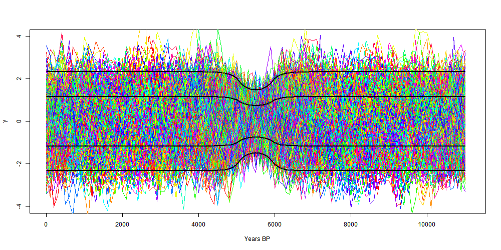
I have now posted three "elementary" emulations of Marcott et al. Each, in its own way, was a year by year average (here, here, and here). As such, it missed the distinctive feature of Marcott et al, which was the smoothing produced by Mante Carlo modelling of the dating uncertainty. So here I am trying to grapple with that.

A story - I used to share a computer system with a group of statisticians. It worked well (for me) for a while - they used Genstat, GLIM etc - no big computing. But then some developed an enthusiasm for Monte Carlo modelling. I've had an aversion to it since. So here, I try to use exact probability integrals instead. There are clearly big benefits in computing time. Marcott et al had to scale their MC back to 1000 repetitions for the Science article, and I'm sure they have big computers. My program takes a few seconds.

A reconstruction is basically a function F(d,t,e) where d is data, t time, and e a vector of random variables. MC modelling means averaging over a thousand or so realizations of e from its joint distribution. But this can also be written as a probability integral:
R(t)=∫F(d,t,e) dΦ(e)
where Φ is the cumulative distribution function.

MC modelling means basically evaluating that integral by the Monte Carlo method. For high dimensionality this is a good alternative, but if the variables separate to give integrals in one or few variables, MC is very inefficient.

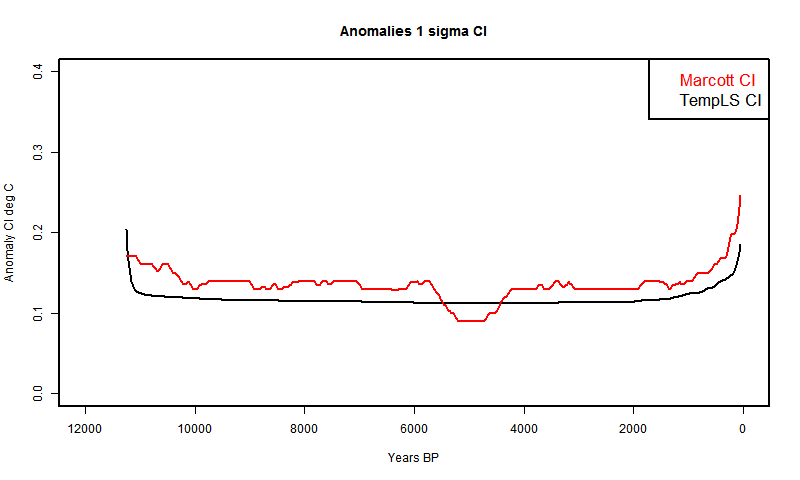
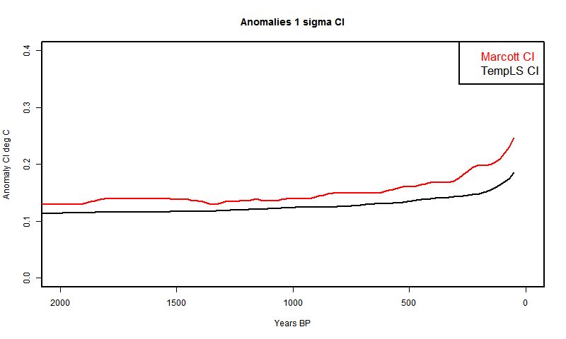
The aim here is to separate the stochastic variables and integrate analytically in single variables. The scope is just to generate the recon - the CI's will wait for another day

Variables, date uncertainty and basis functions

The data consists of a set of proxies calibrated to temperature. There is uncertainty associated with the temperature calibration, and of course there is general variability which will ensure that no reconstruction is exactly fitted; this is modelled as residual noise. For the purpose of calculating the mean recon, these added stochastic variables will in a Monte Carlo converge to their mean, which is zero. So they needn't be included.

The variable that is important is the age (date) uncertainty. This arises from various things - the mixing of material of different ages that may have occurred; reservoir times, meaning that the proxy material may not have actually reached the sampling site for some years, and uncertainty in the actual dating, which is mostly based on Carbon 14.

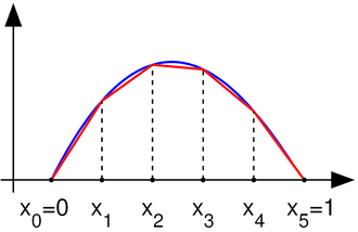
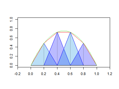
In a post a few days ago, I described how an interpolated function can be described as the product of data values with triangle basis functions. That will be used here. The date uncertainty becomes a stochastic translation of the basis functions.

Random variables

As mentioned above, if the analytic integral approach is to succeed, it will be desirable to partition the variation into items affected by a single (ideally) independent random variable. In fact, for dating an obvious candidate would be the C14 point uncertainty, which affects the data ages through the age model construction. I could not see how to actually do this, and Marcott et al give individual age uncertainties to the data points, as well as C14 uncertainties. Furthermore the data uncertainties are much higher than they would have inherited by interpolation from the C14 points, so I assume other sources of uncertaintyt are included. Still one would not expect the data points to vary independently, but no other information is given. I came to believe that Marcott et al did vary them independently, and in terms of the amount of smoothing that results, it may not matter.

Integrals

I treated the basis functions in the finite element style described in the previous post. That is, I summed them for each proxy by intervals, with two half-triangles at a time. Let a data value f0 is associated with a triangle basis function B01(t) on the range t0 to t1 (where t1 is the next data point), and B01(t)=1-(t-t0)/dt, dt=(t1-t0). If the date uncertainty of t0 is s0, then the probability integral expressing the expected value of product at time t is
∫ f0*B0(1+(t0+s0*e-t)/dt) f(e) de
where f(e) is the unit normal probability density function (Gaussian). The limits of the integral are determined by B being between 1 and 0.

There is a wrinkle here - both t0 and t1 have error, and you might expect that to be reflected in the difference dt. If the error in t1 were independent, then t1 might easily become less than t0 - ie data points would get out of order. However, with age model uncertainty that won't happen; the interpolated data ages will just slide along in parallel, and dt will not vary much at all.

So I thought that a much more reasonable assumption is that B can translate, but not contract.

As mentioned, I sum two parts of the basis on each interval, to make up a linear interpolate. The algebra all works if t0 and t1 are interchanged.

Evaluation

The probability integral is linear in e, and easily worked out:
\[\frac{t1-t}{dt} (\Phi(\frac{t1-t}{\sigma})-\Phi(\frac{t0-t}{\sigma}))
+\frac{\sigma}{dt}(\phi(\frac{t1-t}{\sigma})-\phi(\frac{t0-t}{\sigma}))\]
where Φ is the cumulative normal.

The time values t are Marcott's 20 year intervals, going back from 1940 (10BP) to 11290BP. So this process of smoothed basis functions effects the interpolation on to those points, on which the different proxies are then aggregated.

End conditions

The operation of this integral process is like gaussian smoothing, except that s changes from point to point. So some notion is needed of values beyond the range of proxy data, if it does not extend the full range. This is indeed the bugbear of the analysis.

My first inclination was just to extend the first and last values, although I did not let them go to negative ages BP. That worked fairly well, as I shall show.

First reconstruction

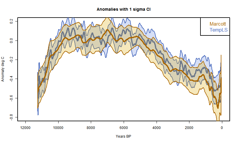
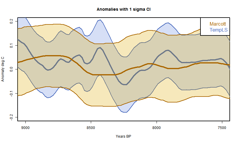
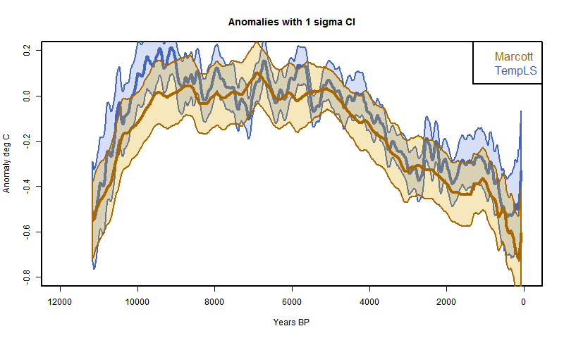
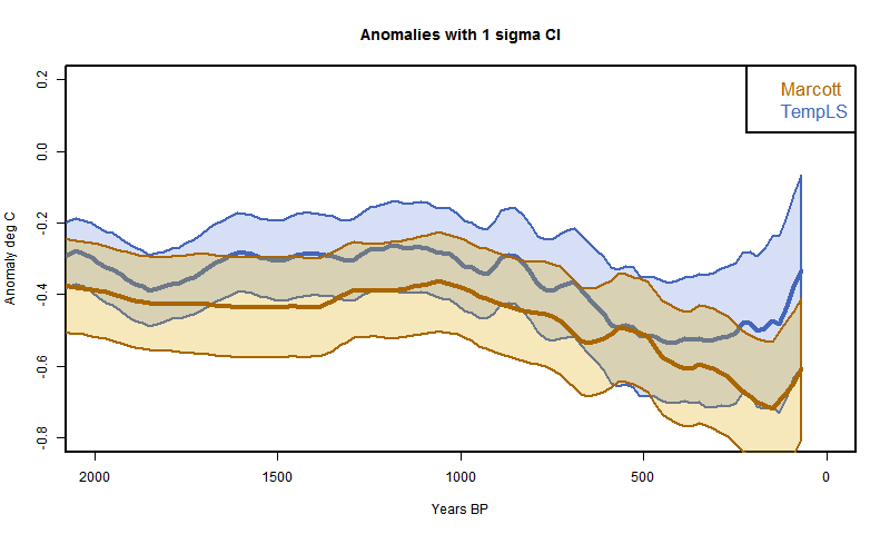
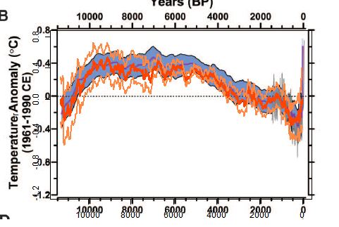
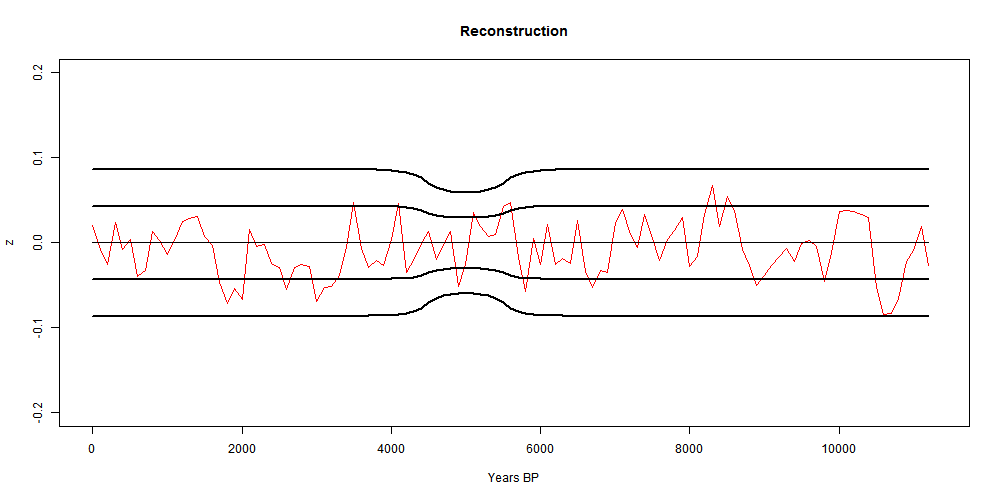
My first recon was much as described here, but with the date process above added. The 73 proxies were located in 5x5° lat/lon cells. Time data at the 20-year intervals was calculated for each proxy. Then cell averages were computed, and then an area-weighted mean (allowing for latitude variation of cell area). At each time point, of course, only the proxies with data are included in the sum, and the weights are adjusted at each 20yr point to allow for missing proxies.

The result was this:


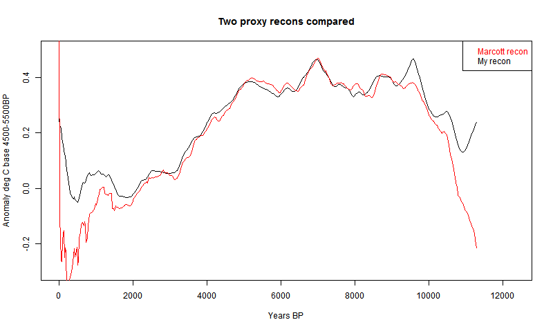
It's mostly quite a good fit, and clearly has about the right degree of smoothing. But it diverges somewhat in early Holocene and much more close to present. This is likely to be due to proxies coming to data endpoints, so I thought a more thorough treatment was required.

Better end treatment

So I looked more carefully at what would happen in a Monte Carlo near data endpoints. At the start, the first age point moves back and forth, so that some of the 20-yr points are sometimes in and sometimes out of the data range. That implies a change in the cross-proxy weighting. When that proxy is considered missing, it's weight goes to zero and other weights rise (to add to 1).

That's bad news for my method, which tries to keep the effect of the random variables isolated to a single proxy data point. This would spread its effect right across.

However, there is another way of allowing for missing data in an average which I find useful. You get exactly the same result if you don't change the weights but replacing the missing value with the (weighted) average of the remaining points. Then the weights don't need to change.

The problem is, we don't have that value yet; we're doing the proxies one by one. The solution is, iteration. The ending proxy is just one of at least fifty. It doesn't make that much difference to the aggregate. If we substitute the numbers from the first recon, say, then the second time around we'll have a much more accurate value. A third iteration is not needed.

There is a subtlety here where there are several in a cell. Then when one goes missing, it should be replaced by the cell average. It is only when the proxy was alone in a cell, that it should be replaced by the recon average when it goes missing. The test is always, what value should it have so that the aggregate would be the same as if the remainder were averaged without it.

Second recon

So I did that. That is, I in effect padded with the recon average from a previous iteration, or the cell average if appropriate. The result was this


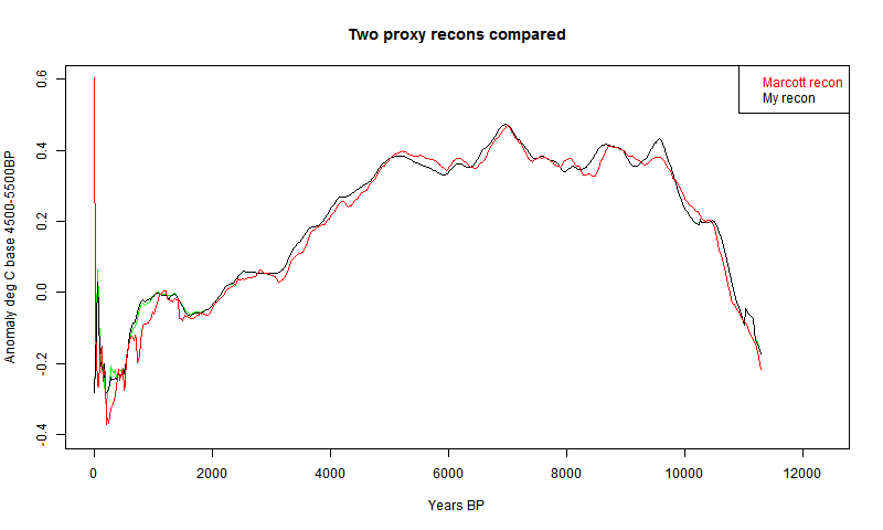
I had previously made an error with the cell area weighting, which affected this plot. Now fixed.
It's much better at the start. In fact, it even almost reproduces Marcott's non-robust 1940 spike (well, after fixing a start problem, it's now a 1900 spike followed by a dive). I fixed a problem at the early end, so that I now use data beyond the end where available in the integral, as Marcott seems to have done with Monte Carlo. So agreement is good there too..


Tuesday, April 23, 2013

March GISS Temp up by 0.10°C


This might be old news - my automatic system had again stopped automatically checking GISS. Anyway GISS LOTI went from 0.49°C in February to 0.59°C in March. Most other measures were fairly steady. Maps below.


Here is the GISS map for March 2013:


And here, with the same scale and color scheme, is the earlier TempLS map:

Previous Months


February
January
December 2012
November
October
September
August
July
June
May
April
March
February
January
December 2011
November
October
September
August 2011

More data and plots


Monday, April 22, 2013

Active viewer for the Pages2K proxies


This viewer is similar to that for the Marcott proxies. It covers the very well presented online data for the new Nature Geosciences paper Continental-scale temperature variability during the past two millennia.

Darren Kaufman has a post on this paper at Real Climate. There are several posts at Climate Audit

Because of the large number of proxies, there are now several different key tables. Each starts with continental regions in black, and you can click on any of these to move to that selection. It may take a few seconds for the new key to appear. Then you can click on any proxy to superimpose a black plot on the background spaghetti plot for that region. The metadata from the online data will show top right, and the location on the map.
The spaghetti plot shows the proxies smoothed with a 21-year moving average filter, and normalized to mean zero, standard deviation 1, over their respective periods. When you select a proxy, it shows the curve in black similarly smoothed and scaled, but the y axis is marked in the appropriate unit. Also shown is the unsmoothed plot in a grey transparent color. Low resolution data has been linearly interpolated.

The swap button allows a blink comparison between the last two proxies selected. These can be from different regions.

Update. I have added a search facility. Above the map there is a text box and a search button. You can enter any text (like "d18"), click the button, and little arrow marks will appear beside each proxy which has that phrase in the metadata. So you can search for types, authors etc. The arrows are cleared before each search, so if you want them to go away, do an unsuccessful search.

It actually searches the underlying HTML, which may give a false positive.


Wednesday, April 17, 2013

Interpolation, proxies and uncertainty


I have now posted three simplified emulations of the Marcott et al reconstruction, here, here, and here. Each used what I believed to be their assumptions, and I got comparable means and CI's. And I think the Marcott assumptions are fairly orthodox in the field.

But I've been wondering about the noise structure, and in particularly the effect of the extensive interpolation used. The proxies typically have century+ resolution, and are interpolated to twenty year intervals.

The interpolated points are treated as independent random variables. They have about the same uncertainty (amplitude) as data points. But they are certainly not independent.

I find it useful to think about interpolation in association with the triangular basis (shape) functions of the finite element method. I'll talk about those, and about the kind of linear model approach to reconstruction that I described in my last post. Below the jump.

Basis (shape) functions

These are described  here. For this context, they are the simplest possible - triangles of unit height. From Wiki, here's a linearly interpolated function:


That has regularly spaced intervals, but that's not at all essential. The corresponding basis functions are shown here:


Wiki doesn't show this well in the diagram, but the interpolate is achieved just by multiplying each basis function by the corresponding data point and adding the results, as shown here:


A major elegance of the finite element method is that you can then switch attention to the elements (intervals) and assemble the result (interpolate) by operating on the fractions of the basis functions that lie with ine element.

Linear model

In the last two posts (here and here.) I have described how the collection of proxy data (Ttp) can be fitted to a simple linear model:
Ttp=Tt+Pp + error
where Tt is the global temperature function being sought and Pp are offsets associated with each proxy (index p). When I did that, the data points were interpolated to 20-year intervals, and that was the spacing of t. So there were 565 Tt parameters over 11300 years.

With 20-year basis functions Bt (τ) you can interpret Tt as a continuous function of time τ:
T(τ)=Σ Tt Bt (τ)
That's the linear interpolate; the Tt are still the parameters we're looking for by fitting.

In principle, I believe you should enter just one equation for each data point, which gives a reasonable chance that the residuals are independent. But how to make that equation?

Collocation

I'll now write s instead of t when thinking about the irregularly spaced data times
You could say just that a data point Tsp stands on its own, and the equation associated with it is:
Tsp=T(s)+Pp + error
T(s) would be expressed as Σ Tt B_t(s)
That looks like potentially a large sum. However, only two at most basis functions overlap s, so only two of the T coefficients are implicitly involved.

However, that would give low weighting in the equation system to proxies that had sparse data values. They may not deserve that, because the data value may be representative of a longer interval. In many cases, sparse proxies are so because it was decided that there just wasn't much point in expressing numbers at finer resolution; they just don't change enough.

Galerkin

The extreme alternative view is to say that the data point is representative of the interval up to the next point. That's really what is assumed when the data is linearly interpolated. In our terms the data point represents a contribution measured by its product with its basis function.

Well, that's OK, but we need numbers. In the Galerkin method, that is obtained by multiplying the continuum proxy equation
Tps Bs(τ)=T(τ)+Pp
by that same basis function Bs(τ) and integrating. The integration is in principle over all time, but the basis function is only non-zero on the intervals adjacent to s.

Implementation

I'm currently trying to implement the Galerkin method. The results are noisy, and I'm not sure if I'm getting it right. I'll report.


Tuesday, April 16, 2013

TempLS-style paleo recon but with biglm


In the previous post, I described the use of TempLS to fit a reconstruction of temperatures during the Holocene, using the data of Marcott et al 2013. It's actually a rather smaller problem that TempLS normally handles, and can be done by the R package biglm. So I wrote a simpler version for which I can supply code.

To briefly review the TempLS style fitting, the model is that the total set of interpolated proxy temperature readings Ttp can be approximated by a global time function Tt and a set of proxy offsets Pp. The system
Ttp=Tt+Pp
has way more equations than variables, but a least squares solution can be found by regression (biglm).

My interest in doing it this way is that I can use it to implement my next project, which is to make the time expression not a discrete set of points but a projection onto a function space, probably trigs. That will give a more consistent treatment of the limited frequency respoonse, and also have many fewer variables (no interpolation)

The results are very similar to the TempLS results; the CI's are those from biglm. Details below the jump. Plots have been added.

In the lm() formula y~x, y is the listing of all interpolated proxy temperatures; there are about 30000 of them. The x matrix of variables is basically an incidence matrix (no weighting is done in this simple program, but a weight vector could be supplied). There are 565 columns for each time step (20 yrs) and 73 columns for the proxy. Each row has a 1 in the column for time and 1 in the column for proxy. The program consists of compiling this, running biglm, and from the summary using the coefficients and se's to make the plots as in the previous post..

I won't repeat the diagrams, they are very similar to the previous post. The code and data (prox.sav) and plots are in this zipfile.

Update - change of mind. The tracking plots are much the same, but less divergence, and the CI plots are notably smoother. Here they are:


And here is the plot with just the CI's for comparison.


Here are versions restricted to the last two millenia.


Sunday, April 14, 2013

TempLS and paleo - Marcott et al


TempLS is a program I wrote for getting global average surface temperature anomalies. I've been using it every month to calculate an index from GHCN/ERSST data, which I compare with GISS when it comes out. It differs from those usually used in that it associates offsets with stations and does a least squares fit, so avoids fittinga fixed anomaly period into station data. The math basis is described here. And here is a somewhat dated overview.

I've been in discussion at Lucia's (see also recent threads here), and it seemed to me that a method she was proposing for anomaly reconstruction for paleo could be implemented in TempLS. Although TempLS is oriented toward monthly data with seasons, it can fix on just one month of the year, so all I had to do was get data in the right input format. As with my earlier recons, I did not attempt the Monte Carlo variation of dating and calibration. I used the published dating.

It works quite well - I'll show early results below. It avoids the dimple. I use the same 5x5 weighting scheme. However TempLS has extensive facilities for weighting by different methods, such as unstructured triangular meshes, which are well suited for sparse sets like these.

Details below.


The Marcott et al data comes from the Supplementary Materials spreadsheet. In these plots I have shifted all curves to a 4500 to 5500 BP anomaly base for plotting. However, I am using the Marcott et al CI's as from the spreadsheet, and the TempLS calc did not use this period, so I did not modify the CI's to reflect this shift. I smoothed all data using a century moving average. This cuts 40 years off each end. The reason I smoothed the Marcott data is that it is given to only two significant figures, so is whiskery when plotted unsmoothed.

Here is the plot over the full period with the TempLS and Marcott reconstruction with shaded CI's. One thing to note is that the TempLS solution is dimple-free. The overlap is fairly good - TempLS strays a bit at the ends. I'm checking for possible reasons.


And here is the plot with just the CI's for comparison. TempLS is mostly lower, but again does not include error due to calibration and dating uncertainty.


Here are versions restricted to the last two millenia.


Saturday, April 13, 2013

Confidence intervals match Marcott et al


In recent days there have been two issues raised at Climate Audit regarding the confidence intervals shown in the proxy reconstruction of Marcott et al. In the first, Romanm claimed that there was a major term missing from the confidence intervals, which could only be remedied by going back to the original calibration experiments and importing the variation of residuals as uncertainties in Marcott's analysis.

And in the second, an issue was made about a "dimple" in the confidence intervals, which in the two previous posts I have shown to be a perfectly natural consequence of the anomaly calculation.

Some weeks ago, I posted an early emulation, without the Monte Carlo variation of dating and calibration, of Marcott's analysis. In this post I will revisit that to show that the confidence intervals calculated purely on between proxy variation match those of Marcott, including the dip.

In Roman's thread, I argued strongly that the variation he said had been excluded was well covered by between proxy variation in the reduction of the 5x5 stack, and that this was the normal way of handling it. I cited Loehle and McCulloch, 2008 which had done this directly. This was apropos, because that paper had been discussed at Climate Audit prior to submission, and met with approval.

The counter was that the description of the stack reduction could be interpreted to say that the between-proxy variation had not been taken into account. I believed though that it must have been; the requirement to do so would have been obvious in the method.

So here I repeat the simple emulation, which is essentially the method of Loehle and Mcculloch. The code is at the end.

Emulation superimposed


In this plot, as in the earlier post, I am using grid weighting as im M13, and the "published dates", so the controversial spike is absent. The standard error of the mean is just the appropriate weighted variance, and this is used in the 1σ CI. The plot is as in my earlier post, except that I am now using the correct 4500:5500BP anomaly base. The CI's of my curve are shown in orange.


Here is the curve and CI's in isolation.


And here are the CI's shown without the curve, mine and Marcott's. My curve lacks the smoothing effect of Marcott's, but you can still see the dimple. But the main thing is that it matches well, and over the central range mine are narrower, despite the lack of smoothing. Marcott et al includes dating and calibration uncertainty.


In the light of this, I am now confident that Marcott included between proxy variation in his CI calc.

Code

There is a zipfile ,a href="https://s3-us-west-1.amazonaws.com/www.moyhu.org/misc/peru/dimple.zip">here
with code and data.

# A program written by Nick Stokes www.moyhu.blogspot.com, to emulate a 5x5 recon from
#A Reconstruction of Regional and Global Temperature for the Past 11,300 Years
# Shaun A. Marcott, Jeremy D. Shakun, Peter U. Clark, and Alan C. Mix
#Science 8 March 2013: 339 (6124), 1198-1201. [DOI:10.1126/science.1228026]
#https://www.sciencemag.org/content/339/6124/1198.abstract

# Need this package:
getxls=T # set to T if you need to read the XL file directly
if(getxls) library("xlsReadWrite")
# The spreadsheet is at this URL "https://www.sciencemag.org/content/suppl/2013/03/07/339.6124.1198.DC1/Marcott.SM.database.S1.xlsx"
# Unfortunately it can't be downloaded and used directly because the R package can't read the format. You need to open it in Excel or OpenOffice and save in an older format.

loc="Marcott.SM.database.S1.xls"
prox=list()
# Read the lat/lon data
if(getxls){
lat=read.xls(loc,sheet=2,from=2,naStrings="NaN",colClasses="numeric")[2:77,5:6]
} else load("prox.sav") # If the XL file has already been read
o=is.na(lat[,1])
lat=as.matrix(lat[!o,])
w=rep(0,36*72)
wu=1:73; k=1;
for(i in 1:73){
j=lat[i,]%/%5;
j=j[1]+j[2]*36+1297;
if(w[j]==0){w[j]=k;k=k+1;}
wu[i]=w[j];
}
# Read and linearly interpolate data in 20 yr intervals (from 1940)
m=11300/20
tm=1:m*20-10
g=list()
h=NULL
source("CI.txt")
if(getxls){
for(i in 1:73){
prox[[i]]=read.xls(loc,sheet=i+4,from=2,naStrings="NaN",colClasses="numeric")[,5:6]
}
save(prox,lat,file="prox.sav")
}

for(i in 1:73){ # Anomalize
u=prox[[i]]
g[[i]]=approx(u[[1]],u[[2]],xout=tm) # R's linear int
y=g[[i]]$y
y=y-mean(y[-25:25+250]) # anomaly to 5800-6200 BP
h=cbind(h,y)
}
r=rs=NULL # Will be the recon
# now the tricky 5x5 weighting - different for each time step
for(i in 1:nrow(h)){ # loop over time
o=!is.na(h[i,]) # marks the data this year
g=h[i,o];
u=wu[o]; n=match(u,u); a=table(n); d=as.numeric(names(a));
e=u;e[d]=a;wt=1/e[n]; #wt=weights
wt=wt/sum(wt)
# calc mean and variance
mn=sum(g*wt)
va=sum((wt*(g-mn))^2)
# Accumulate mean and CI
r=c(r,mn)
rs=c(rs,sqrt(va))
}
# Now standardize to 1961-90, but via using M et al value = -0.04 at 1950 BP
r=r-r[98]-0.04
# now tricky graphics. my.png is the recon. ma.png is cut from fig 1b of the paper. You have to cut it exactly as shown to get the alignment right
ch="#ff8844"
png("myrec0.png",width=450,height=370)
par(bg="#ffffff00") # The transparent background
par(mar=c(6,5,3,0.5))
plot(tm,r,type="l",xlim=c(11300,0),ylim=c(-1.2,0.8),col="#ff4400",lwd=3,yaxp=c(-1.2,0.8,5))
lines(tm,r+rs,lwd=2,col=ch)
lines(tm,r-rs,lwd=2,col=ch)
dev.off()
png("myrec_0.png",width=450,height=370)
par(bg="#ffffff00") # The transparent background
par(mar=c(6,5,3,0.5))
plot(tm,r,type="n",xlim=c(11300,0),ylim=c(-0.5,0.5),col="#ff4400",lwd=3,yaxp=c(-1.2,0.8,5))
lines(tm,rs,lwd=2,col=ch)
lines(tm,-rs,lwd=2,col=ch)
lines(tm,un,lwd=2,col=3)
lines(tm,-un,lwd=2,col=3)
dev.off()
# Now an ImageMagick command to superpose the pngs
# You can skip this if you don't have IM (but you should)
system("composite myrec0.png ma.png reco0.png")


Friday, April 12, 2013

A proper uncertainty dimple


In my previous post I discussed proxy reconstructions, anomalies and uncertainties. I looked at a stochastic model for a single proxy, and derived an expression for the CI. This was (1σ):
+- sqrt(DKD*) where D is a simple matrix which implements the mean subtraction step of anomaly formation and K is the covariance matrix of the time sequence residuals.

I have now applied this to the case of AR(1) residuals. This gives a pattern similar to the Marcott case discussed at Climate Audit. There's a bonus in that fitting the shape gives an estimate of the AR(1) lag factor.
#Update - section relating this model to recon, and R code added

I used the same general scheme as in the previous post to generate the AR(1) sequences. I set the scale to match the Marcott plot in century steps. Here is that plot from Climate Audit:


I actually used the DKD product to compute, though an analytic expression can be derived. With r=0.6 in century units, I plotted 700 proxy realizations, plus the 1σ and 2σ bounds. I've scaled so that the 2σ look like the shape of the Marcott 1σ, but doubling the scale would match the 1σ shapes. Here's the plot:


The scale is reversed, but it is symmetric. I think both the shape and depth of the dip match fairly well for r=0.6.


Update - fun fact.
The dimple has an analytic form for AR(1), parameter r, at least if the base region has an odd number of points M. It is:
Let m=(M-1)/2, i be the time index centered at the middle of the base
Let y0=(1+r)*(1-2*r/(1-r^2)*r9/M)
If i≤m (i in base): k_i=r^|i-m}-r^|m+i+1|
If i>m:  k_i=1+r-r^(m+i)-r^(m-i)
Then variance y_i=1+(y0-2*k)/M/(1-r)

The function is like a cosh in the base, then asymptotes exponential to the far field.

Noise model and proxy reconstruction

In this post, I've stripped the mathematics down to just a noise model AR(1). I should review how that relates to a proxy reconstruction.

I've drawn 700 realizations of that noise in the plot. You could think of a toy recon in which 700 proxies around the world, some hot, some cold have a fixed base temperature, with one of those noise realisations added.

So we'll make a reconstruction from these. We take anomnalies (using D). This strips out the varying fixed base temperatures, and leaves 700 realisations of anomalised noise, which will each have the CI's shown here.

Then we average them. That will be the recon. The CI's are scaled down by sqrt(700), leading to this plot:


Code

#Code written to calculate for CIs of an anomaly calculation, AR(1) noise
#Nick Stokes www.moyhu.blogspot.com 13/4/13

# Set up covariance matrix K for AR(1)
r=0.6 # AR(1) parameter
X=113 # timesteps
x=1:X-1 # timescale
K=r^(abs(outer(-x,x,"+")))
# Set up anomaly op
base=45:55+1; M=length(base);
D=K*0; D[,base]=1/M; D=diag(X)-D;
# Matrix products to get variance
E=D%*%(K%*%t(D))
ci=sqrt(diag(E)) # variances
#Analysis complete
# Now plot sigma and 2*sigma CI's
x=x*100 # rescale to years
png("dimple.png",width=1000, height=500)
plot(x,ci,xlim=c(0,X*100),ylim=c(-4,4),type="n",xlab="Years BP")
# Now make proxies for plotting
cl=rainbow(22)
h=range(base-1.5)*100
rect(h[1],-4,h[2],4)
for(i in 1:100){
u=as.vector(arima.sim(n=X,list(order=c(1,0,0),ar=r),sd=sqrt(1-r^2)))
lines(x,u-mean(u[base]),col=cl[i%%22+1]) # proxy curves
}
for(i in -2:2)lines(x,i*ci,lwd=(i!=0)+1) # CI curves
dev.off()

Thursday, April 11, 2013

Reconstructions, anomalies and confidence intervals


There has been discussion recently of the confidence intervals of the Holocene temperature reconstruction of Marcott et al. I've been posting a lot on this paper recently, here, here, here, and here. So have others, and I got involved in a discussion at Climate Audit. There they noted a dip in Marcott's confidence intervals at about the period of his anomaly base (4500-5500 BP). BP means before present, taken to be 1950. The discussion went on to Lucia's where I believe there is a post on the way.

So I want here to review first what reconstructions are trying to do, why anomalies are needed, why they are often done with subsets of the available time as base, and why this inevitably causes a "dimple" in the CI's.


Reconstructions.

So we have a set of estimated temperatures over various time periods in the past. Marcott's are typical. Usually in a multi-proxy recon, they are of diverse types and come from a mixture of places that are hot, cold and in between.

There has been much discussion of tree-ring and other proxies that require calibration to instrumental observations. Marcott's don't, and I'm going to skip this complication.

In fact, the formation of a global instrumental temperature index has essentially the same issues, and is more familiar and better established.

So we have a bunch of time sequences and want to express the variation that they have in common.

Naive Reconstruction.

So why not just average? Well, partly there's the question of, what does it mean to average, with Marcott, a whole lot of ice core and marine/lake environments. Does that give a world average?

Most organisations that provide surface temperature indices don't do this. GISS explains why, also NOAA.

About the only exception that I am aware of is that for historic reasons (I think) the NOAA produces average US figures. This is typical of the problems it can cause. There are actually two networks, USHCN and CRN. They produce two different average temperatures. The linked post argues that the new network, CRN, is better and shows cooler temps than USHCN did many years ago, so the US must be getting cooler. But it turns out that CRN is on average higher, so the temperatures are bound to be cooler. Which is right? You can argue for ever about that.

Here's another indicator of the silliness that can result. The claim is that to make the globe temp look warmer, the NOAA through GHCN had been selectively eliminating cool climate stations.

Now in fact cool regions of NH particularly had been over-represented. That doesn't matter too much; gridding takes care of it, mostly. But it matters even less because anomalies are used - ie temperatures with ref to some average. So even without gridding a shift in station climates has little effect.

That's the key reason for a move to anomalies - absolute temperature averages depend absolutely on the stations in the mix, and if stations go missing for whatever reason, the average shifts.

Anomaly reconstructions

One good thing about anomalies is that they vary smoothly over space. You can see that by leafing through the maps here. That makes it possible to sum in a way that approximates a spatial integral. A spatially averaged anomaly reconstructions should be made up of a weighted average which best emulates an integral.

But the key benefit of using anomalies is that they minimise the effect of missing data. All stations in the sum have expected anomaly value close to zero. If an anomaly is missing, its effect on the average is as if it had the same value as that average, which is not likely o be far wrong.

The "dimple" which I will discuss is not likely to be visible if the anomaly is taken with respect to the average of the data for each proxy. But there is a good reason to use a common base period, as all the major surface indices do. Using different periods for different proxies can affect the trend.

Here's an example. Suppose just two stations, A and B. both with just a linear temp history. A has a record from 1900 to 1975, and rises from -1°C to 0.5°C. B goes from -0.5°C in 1825 to 1°C in 2000. As you'll see they have the same temps from 1926 to 1975, and a trend of 2°C/Century, and are both 0 in 1950.

If you use 1925-1975 as the anomaly base period, 0 is added to each, and the recon is just the line from -1 in 1900 to 1 in 2000, a slope of 2 as expected.


But if you use the whole period, averaging where data exists, then 0.25 is added to A, which then goes from -0.75 in 1900 to 0.75 in 1975. And 0.25 is subtracted from Bm, which goes from -0.75 in 1925 to 0.75 in 2000. The trend is now 1.333 °C/Cen.


The simplest solution is to find a range where all proxies have data to use as a base. This is what Marcott et al did, using 4500-5500 BP. For surface stations, more elaborate algorithms are required, which generally take advantage of the greater density of stations.

Confidence intervals

The reconstruction is a mean across proxies, and the natural measure of uncertainty is the pointwise standard error of that mean. That is what was used in, say, Loehle and McCulloch (see p 95). And it seems to be the main part of the Marcott calculation, which also incorporates Monte Carlo variation for date and calibration uncertainty. I say seems, because their description is noy entirely clear, and the linked CA post seems to interpret as not including variability of the mean. But that would be a strange thing to do when they calculate that mean.

Marcott et al show 1σ levels, so I will use that convention.

Toy example

I'm going to use a linear algebra description, with indices and summation convention (a repeated index is summed over its range). Suppose we have P identical proxies, each from a distribution with an expected value zero and random part &deltapt. p is an index over proxies, t over time (N steps). The toy naive recon is
Tt=wpδpt
where the w's are the weights. I'll assume they are all 1/P, but the term is kept here to carry the suffix to show summation. However I'll now shift to saying that the δs are from the same distribution over p, so the upshot is that the CI for T is sd(δ).

Now in this case we have so many suppositions that there's no reason to take anomalies, but I want to show the effect of doing so. And I want to present it in linear algebra form, Taking as anomaly over a block of M time steps is equivalent to multiplying by a NxN matrix D, made by subtracting from the identity a matrix with M columns comtaining 1/M, zero elsewhere.

Then if the covariance matrix of δ is K, the covariance matrix of the anomalised sequence will be DKD* (* is transpose). The CI's will be the square roots of the diagonals of that matrix.

If the δs had been unit white noise, K would be the identity, and it is left to the reader to verify that the diagonals of DKD* are 1+1/M outside the block of M (anomaly base) and 1-1/M within. I've shown that in two alternative ways here and here (note correction here, which suffered thread drift). That's the dip.

More interesting is the case with AR(1) noise, parameter r. Then the matrix Kij = r^|i-j|. I'll work out the general for,\m in the morning, but I want for the moment to show the interesting particular case when M=1. This has caused a lot of discussion, because the uncertainty goes to zero. Some people cannot believe that, but it is a simple consequence of the fact that the anomaly definition guarantees that you will have a zero there.

In the case of white noise, that can seem like a semantic argument, but with AR(1) it's real. Layman Lurker at Lucia's calculated the case r=0.95. I want to show the theoretical CI's, to show how they tend to zero - this is real arithmetic, not just arguing about definitions.

When you work out the DKD* product now, the diagonal is just 2*(1-r^|i-i0|), where i0 is the anomaly base point. And again, the CI's are the sqrt. Here it is plotted with both 1σ and 2σ CI's. I've taken P=70, as Layman Lurker did - you might like to compare with his plot.


Here's a closeup of the anomaly base region


To be continued.


Wednesday, April 10, 2013

TempLS global temp down 0.05°C in March

The TempLS monthly anomaly for March 2013 was 0.396°C, down slightly from 0.447° in February. I had actually reported a small decrease from Jan to Feb which with more data was converted to a small rise.

Satellite indices also show little change, after a bumpy few months.

Here is the spherical harmonics plot of the temperature distribution:


Europe and N Russia very cold, central Asia very warm.
And here is the map of stations reporting:


Monday, April 8, 2013

Quelccaya icecore and regional temperatures


Prof Lonnie Thompson and colleagues have a new paper in Science Express called "Annually Resolved Ice Core Records of Tropical Climate Variability Over the Past 1800 Years". With annual resolution it becomes worthwhile to compare with measured surface temperatures. I did this with TempLS, using GHCN/ERSST and restricting to an area 1000 km around the location of the Quelccaya site in Peru. The Quelccaya data is here.

This is done partly in response to a thread at Climate Audit, where there was speculation about the possible relationship of the d18O proxy to surface temperature. The standard TempLS analysis is below the step.


The analysis runs from 1900 to 2009. Since Thompson uses the "thermal year" starting for SH in July, I have followed that convention. So what is marked as 2009 is actually Jul 2009-Jun 2010.

Here is a map of all the GHCN/ERSST stations within the radius. ERSST "stations" are the 5x5 lat/lon grid points of the data. The map includes all stations that have reported from 1900-2013, many for only short times. The Quelccaya site is shown with a big blue dot.


Next is a plot of the numbers of stations reporting in each year (for at least 8 months)


Finally, here is the plot of surface temperatures (black) vs Quelccaya d18O. I normalised the d180 data by matching the mean and sd over base 1961-90 to the temperature measure.


Note that the scaling is not to be relied on as I did it by matching. For the first fifty years (with rather small station numbers), there are indications of correlation, but some sranger things recently. The big dip in 1999 in d18O does not seem related to this measure of local temperature. However land temperatures were actually cold, but the 1000 km radius picks up a lot of ocean, which was warm.